Lab 1 Report
January 28, 2019
Comparison of Alcohol Users and Non-users
In this exercise, we will attempt to provide an answer to the question, “How do light users of alcohol differ from those who are heavy users of alcohol in terms of their self-reported overall health?” In this document we will:
- load our data
- make a definition of “light users” and “heavy users”
- filter our data to create two new, smaller datasets: a “light users” dataset and a “heavy users” dataset
- combine those two datasets
- prepare a large variety of graphs displaying the distribution of self-reported overall health of both groups
- report the results
- give several possible conclusions based on these results
Our group will compare people who use alcohol to people who do not use alcohol. We will compare the distribution of Non-users, Light Users, Moderate Users, and Heavy Users. Finally, we will illustrate the difference of heavy alcohol users to light alcohol users.
Our central goal is to illustrate the frequency of alcohol use overall as well as illustrate how the severity of alcohol use differs within alcohol users. We also want to determine if heavy users of alcohol are less healthy than light users.
For the purposes of this data, we will define the following terms:
A Current User is a person who has used alcohol in the past 30 days. A Former User is a person who has not used alcohol in the past 30 days. A Non-user is a person who has not used alcohol in their lifetime. A Light User is a person who has drank less than 10 days in the past month. A Moderate User is a person who has drank between 10 and 20 days in the past month. A Heavy User is a person who has drank over 20 days in the past month. Health is a self-reported variable.
Data
Data is from the National Survey on Drug Use and Health , which is conducted annually by the Substance Abuse and Mental Health Services Administration (SAMHSA), an agency in the U.S. Department of Health and Human Services (DHHS). More information about this survey can be found at ICPSR’s data archive page. The data has been prepared into a .Rdata file, so we can simply load it in the workspace with the load() command. At this time, we’ll also load our packages:
library(tidyverse)
library(forcats)
library(rsconnect)
load("36361-0001-Data.rda")
Because the data object has an unpleasant name, da36361.0001, we make a copy with the name full_data and remove the original data object.
full_data <- da36361.0001
remove(da36361.0001)
Definition of “Light User”
We have defined light users as those who have drank alcohol 10 days or less within the past month.
light_use_criteria <- 10Definition of “Heavy User”
We have defined heavy users as those who have drank alcohol more than 20 days within the past month.
heavy_use_criteria <- 20Data Manipulation
We are looking for the self-reported overall health of people who are categorized as “heavy,” “light,” “moderate,” or “never” users. Below we have manipulated the data to classify people under these definitions using the variable alc_user_status.
full_data <- mutate(full_data, alc_user_status =
                    ifelse(ALCFLAG == "(0) Never used (IRALCRC = 9)", "Never User",
                           ifelse(ALCMON == "(0) Did not use in the past month (IRALCRC = 2-3,0)",
                                  "Former User", "Current User")))
full_data <- mutate(full_data, alc_30day_use = cut(ALCDAYS, c(0, 10, 20, 30),
                                                   c("Light User", "Moderate User", "Heavy User")))

full_data <- mutate(full_data, alc_user_status = ifelse(alc_user_status =="Current User",
                                                        as.character(alc_30day_use), alc_user_status))

full_data <- filter(full_data, !is.na(alc_user_status), !is.na(HEALTH))

full_data <- mutate(full_data, alc_user_status = as.factor(alc_user_status))

full_data <- mutate(full_data, alc_user_status = fct_relevel(alc_user_status,
                                                            "Never User",
                                                            "Light User",
                                                            "Moderate User",
                                                            "Heavy User"))
Using these definitions, we can now create two data subgroups: heavy users and light users. Now, we wish to compare the relative health of people who we have defined as heavy users versus those we have defined as light users.
heavy_users <- filter(full_data, ALCDAYS > heavy_use_criteria)
light_users <- filter(full_data, ALCDAYS < light_use_criteria)
Next, we remove the full_data object and drop the unneeded variables from our light_users and heavy_users datasets. These steps are not necessary, but clearing out unneeded objects and variables can improve the speed with with your code is executed.
heavy_users <- select(heavy_users, HEALTH)
light_users <- select(light_users, HEALTH)
It may be useful to us to have the data about both groups (heavy and light users) in our data object. To accomplish this, we add a new variable user_status to both our data objects. For all observations in heavy_users we wish to set the value of this variable to “heavy” For all observations in light_users we wish to set the value of this variable to “light” Once we have added this variable to both datasets, we combine them using the rbind() function. rbind() stands for row bind – it binds or glues two datasets together along by putting one dataset on top of the other.
heavy_users$alc_user_status <- "heavy"
light_users$alc_user_status <- "light"
combined_data <- rbind(heavy_users, light_users)
Graphs
We start our graphical analysis by making a some basic plots showing the self-reported overall health of regular users.
ggplot(full_data)+
  geom_bar(aes(x=alc_user_status, fill=HEALTH),position="fill")+
  scale_x_discrete(name="Use of Alcohol",labels=c("Never User",
                            "Former User",
                            "Light Current User\n(10 or fewer days per month)",
                            "Moderate Current User\n(11-20 days per month)",
                            "Heavy Current User\n(more than 20 days per month)"))+
  scale_fill_brewer(palette="RdYlGn",direction=-1,
                    labels=c("Excellent","Very Good","Good","Fair","Poor"),
                    name="Self-Reported \nOverall Health")+
  coord_flip()+labs(y="Proportion",title="Self-Reported Health by Marijuana User Status")+
  theme_classic()
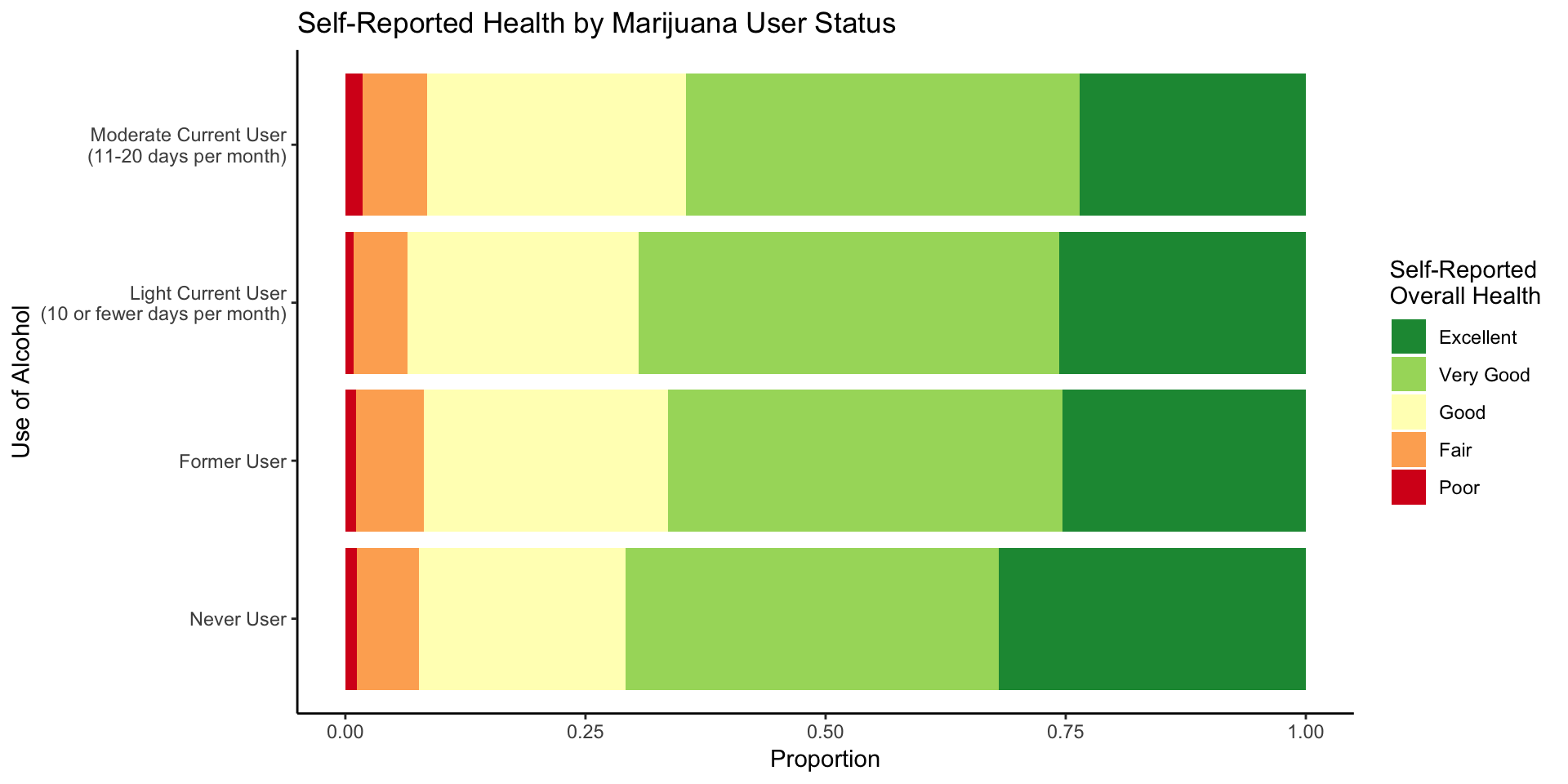
Figure 1: Comparison of self-reported health among “never,” “light,” “moderate,” and “heavy” users of alcohol.
This graph displays the self-reported overall health of people who are categorized as “never,” “light,” “moderate,” or “heavy” users.
Now, we wish to compare the relative health of people who we have defined as heavy users versus those we have defined as light users. We defined heavy users as those who have drank alcohol 30 days within the past month (30 days) and light users as those who have drank 10 days within the past month.
Bar Graphs Comparing Heavy and Heavy Users
ggplot(combined_data)+
  geom_bar(aes(x=HEALTH, fill=HEALTH, y=(..count..)/tapply(..count..,..PANEL..,sum)[..PANEL..]))+scale_fill_brewer(palette="RdYlGn", direction=-1,labels=c("Excellent", "Very Good", "Good", "Fair", "Poor"), name="Self-Reported \nOverall Health")+
  labs(x="", y="Relative Frequency", title="Self-Reported Health by User Status")+scale_x_discrete(labels=c("Excellent", "Very Good", "Good", "Fair", "Poor"))+facet_wrap("alc_user_status")+theme_classic()
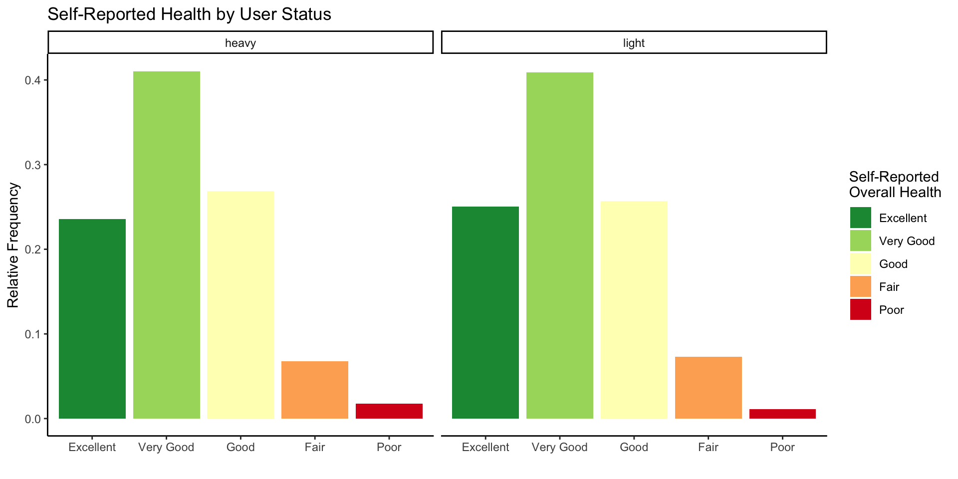
Figure 2: Bar graph comparing the number of times a heavy or light user categorized their health as “poor,” “fair,” “good,” “very good,” and “excellent.”
Pie Chart Comparing Heavy and Light Users
ggplot(combined_data) + geom_bar(aes(x=0, fill=HEALTH, y=..count../tapply(..count..,..PANEL..,sum)[..PANEL..]))+ coord_polar(theta="y") + scale_fill_brewer(palette="RdYlGn", direction =-1, labels=c("Excellent", "Very Good", "Good", "Fair", "Poor"), name="Self-Reported \nOverall Health")+
labs(x="", y="Relative Frequency", title="Self-Reported Health by User Status") +facet_wrap("alc_user_status")+theme_classic()
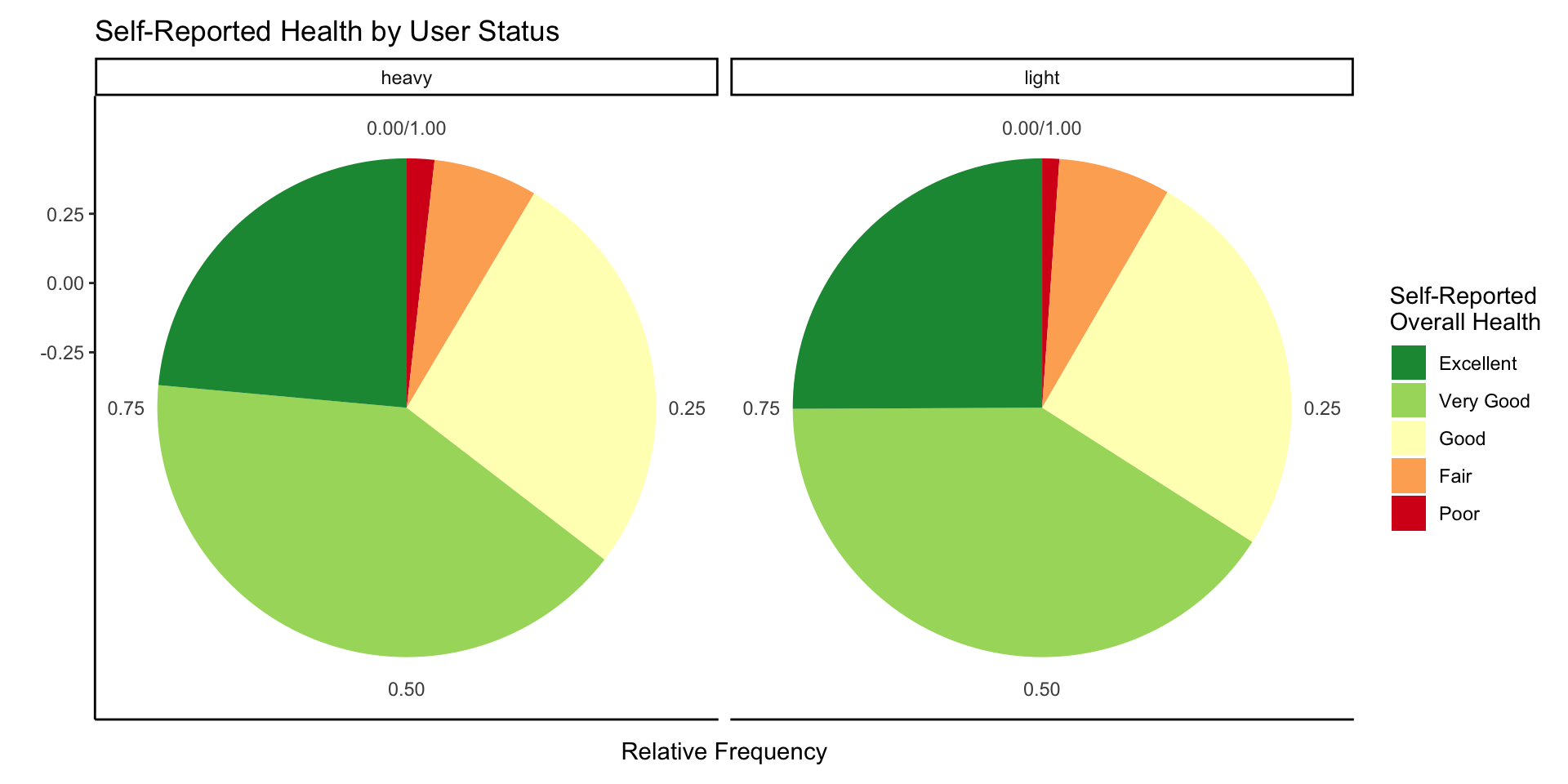
Figure 3: Pie chart comparing percentages of heavy users and light users reporting health on the scale of “poor,” “fair,” “good,” “very good,” and “excellent”
Stacked Bar Plot Comparison of Heavy and Light Users
ggplot(combined_data)+geom_bar(aes(x=alc_user_status, fill=HEALTH),position="fill")+scale_fill_brewer(palette="RdYlGn", direction=-1, labels=c("Excellent", "Very Good", "Good", "Fair", "Poor"), name="Self-Reported \nOverall Health") + labs(x="User Status", y="Relative Frequency", title="Self Reported Health by User Status")+scale_x_discrete(labels=c("Heavy Users", "Light Users"))+theme_classic()
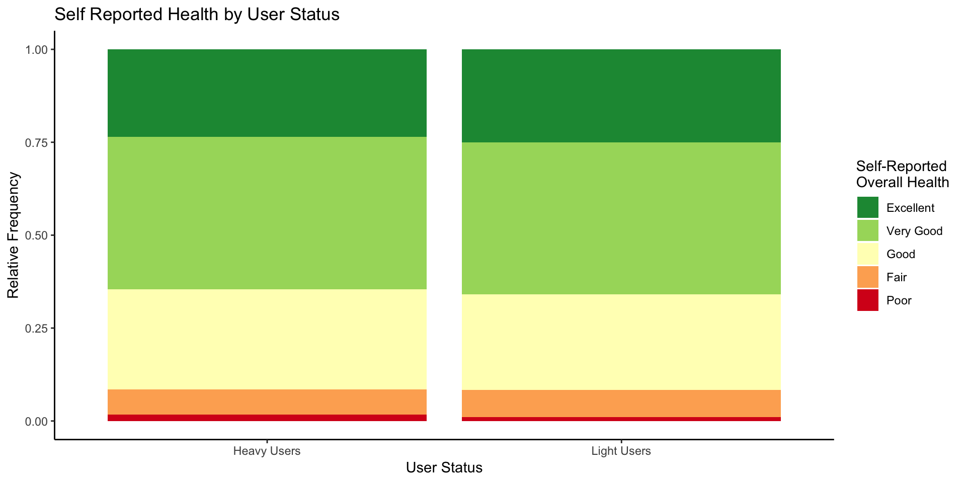
Figure 4: Stacked bar plot comparing the number of times a heavy or light user categorized their health as “poor,” “fair,” “good,” “very good,” and “excellent.”
Numerical Verifcation
user_counts <- count(combined_data,alc_user_status)
health_counts <- count(combined_data,alc_user_status,HEALTH)
#print(user_counts)
#print(health_counts,n=nrow(health_counts))
Manually, we see that 488 of 2072 (about 24%) “heavy users” self-reported “excellent” overall health, which is consistent with what our display shows.
Results
From Figure 1, we can see that heavy users of alcohol were the most likely to self-report their health status as “poor.” Heavy users were also the most likely to self-report their health status as “fair” and the least likely to self-report their health status as “excellent.” People who never used alcohol were the most likely to self-report their health status as “excellent.”
For the purposes of our investigation, we wanted to focus on the differences between the two subsets of heavy alcohol users, which are people who drank alcohol over 20 times in the past month, and light alcohol users, which are people who drank alcohol 10 or less times in the past month. The next three graphs juxtapose these subsets of the data using a bar graph (Figure 2), a pie chart (Figure 3), and a stacked bar plot (Figure 4).
Using side-by-side displays of bar graphs, pie graphs, and stacked bar plot graphs comparing the health of heavy users and light users of alcohol, there does not appear to be much of a difference in the percentages of health reported by heavy and light users. In comparison of health statistics, we deemed it more important to analyze the statistics of reporting on the extremes of the health spectrum: the frequency of reports of “Excellent” health and the frequency of reports of “Poor” health.
Figures 2 through 4 show that overall, heavy users of alcohol and light users of alcohol self-report their health relatively similarly. In other words, heavy users of alcohol and light users of alcohol self-report their health as “fair,” “good,” and “very good” at nearly identical frequencies. For reference, heavy and light users self-report their health as “fair” 7% and 7% of the time, respectively. Heavy and light users self-report their health as “good” 27% and 26% of the time, respectively. Heavy and light users self-report their health as “very good” 41% and 41% of the time, respectively.
However, heavy users and light users self-report their health as “excellent” and “poor” at different levels. Heavy users are more likely to self-report their health as “poor,” while light users are more likely to self-report their health as “excellent.” For reference, heavy and light users self-report their health as “poor” 2% and 1% of the time, respectively. Heavy and light users self-report their health as “excellent” 24% and 25% of the time, respectively.
Conclusion/Discussion
According to the data, heavy users of alcohol are more likely to report “poor” health than any other user category specified. Additionally, in terms of the target groups–heavy and light users–the only statistically significant difference is a small disparity in reporting of poor health. Otherwise, the differences in percentages of reported “fair,” “good,” “very good,” and “excellent” among the two groups are inconsequential, implying that the difference in health among heavy and light users is insignificant. Thus, the data do not suggest that light drinkers are generally more healthy than heavy drinkers.
However, it is important to recognize the limitations of the data. Firstly, it is difficult to confirm the health status of individuals, as self-reported data can be unreliable due to psychological factors affecting people’s perception of their own health. If the health status was not based on self-reporting but instead on quantitative factors, such as the rate of medicine processing in the liver or the number of mental health issues developed since becoming a heavy alcohol drinker, the data could be more reliable. This could help differentiate between how one is “feeling” versus how physically and mentally fit their body is, as a concrete definition of “health” is lacking from the data codebook. Secondly, the amount of reported heavy users (2072 people) is significantly less than the amount of reported light drinkers (17735 people). The analysis would be better if the sample sizes of the light and heavy user categories were either similar or exactly the same.